Script Monkey – The Power of Excel

Script Monkey management has unparalleled Excel experience stretching back to 1990.

We have experience of writing DLL’s in VB.NET for Excel, endless hours of VBA coding and the most detailed experience of using Excel formulas in engineering and construction contexts.

No matter the complexity of your issue, we can help you solve it.

We are always surprised how many companies use Excel for business-critical activities, yet so not have their data or Excel sheets structured in the proper fashion. For this reason, we thought we’d give a little tutorial on how to use a generally unknown function that will revolutionise the way you use Excel…

Introduction to the VLOOKUP function in Excel

VLOOKUP is a little-known function in Excel that will revolutionise how you work. It can be used to find data in another place and return data stored by that thing.

Imagine you are running a small business selling products direct to customers and you have created an invoice/receipt sheet. Elsewhere you have your price list saved in an Excel sheet.

When you are in your invoice sheet, you want to be able to type your product code and then have the Excel sheet find the product description and the price for that item without you having to do it. This is surprisingly easy...

How is this magic achieved?

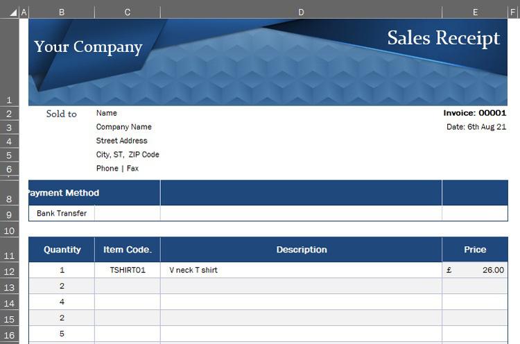
Create an Excel file called invoice01.xlsx and save it to desktop for now…

Format this file to suit your business. We used an Excel template from the net. In Excel, select the File menu and choose New and pick an invoice type template. Then make it look the way you want. In this case, we left it all empty, but added some quantities for the first five lines.

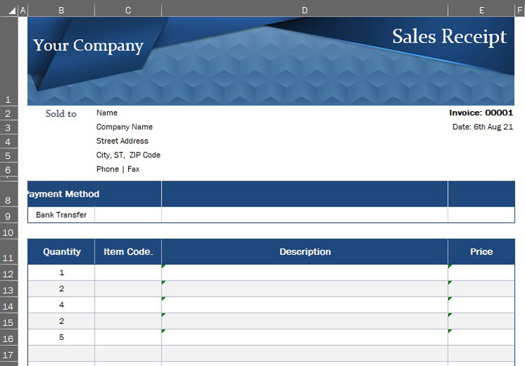
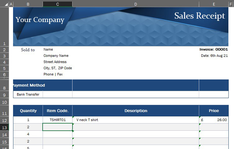
Now, just imagine you can type in your product code, say TSHIRT01 into the cell C12 and press enter, and the sheet would automatically look up the product and get the description and price for you from a central price list. you only update your prices, and all of your invoices update themselves automatically! Let's do this

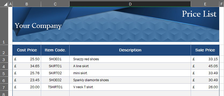
First, create another Excel file called pricelist.xlsx, name the first tab to 'Price List' (without quotes) and save it to the same place you saved the invoice01.xlsx file. We have populated the sheet below with some products and have used cost price, product code, description, and sales price columns.

Now in cell D12, type: =VLOOKUP(C12,'C:\[type your path here]\[pricelist.xlsx]Price List'!$C$3:$E$7,2,FALSE)

If you are not sure what path to type, you can get this from the address bar in the file explorer, or Excel can fill this in for you...

If you can't get the path on your machine, make sure the pricelist.xlsx file is open and type: =VLOOKUP(C12, and then click on the pricelist window with your mouse and drag your mouse from cell C3 to cell E7 so a rectangle is highlighted. Excel will fill in the path for you, then continue to type: ,2,FALSE)

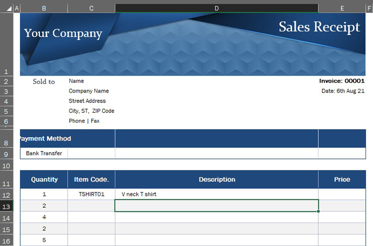
Don't worry, we will break this down in a bit, but for now, just try it and you will see that the description is now filled in on the invoice from the pricelist file.

Now in cell E12, type: =VLOOKUP(C12,'C:\[type your path here]\[pricelist.xlsx]Price List'!$C$3:$E$7,3,FALSE)*B12

Excel will get the price from the pricelist file and multiple it by the quantity we typed to give a sales price.

Now if we highlight cells D12 and E12 and press Ctrl+C (Copy), then highlight cells D13 to E16, right-click and choose Paste Special and formulas, we get the VLOOKUP formulas copied and will see this:

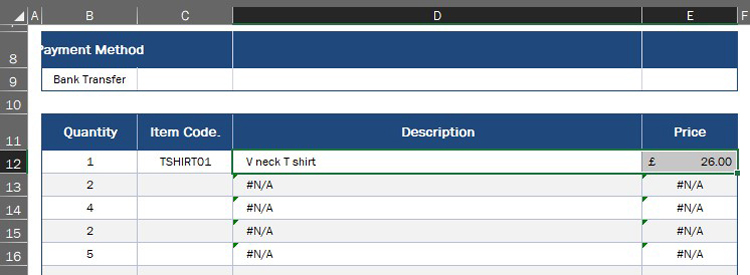
A couple of things to note here: We used a dollar sign before the $C$3:$E$7 inside the VLOOKUP function - this is because when we copy it to other cells, we did not want the cells C3:E7 to change as Excel copied our formulas. This is important and you should look at how Excel uses a dollar sign to fix references, then you will have ninja power!. One other thing of note is that if we do not type a product code, we get a #N/A from VLOOKUP which is ugly.

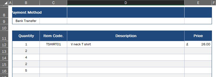
To cure the #N/A which is a VLOOKUP error meaning 'I cannot find a match for nothing', we wrap the IFERROR function around VLOOKUP and tell it to return a blank string ("") if VLOOKUP fails. We do that like this:

In D12 modify the cells to be like this =IFERROR(VLOOKUP(C12,'C:\[type your path here]\[pricelist.xlsx]Price List'!$C$3:$E$7,2,FALSE), "")

Now without product codes in our invoice we stull get a tidy result if we add IFERROR to E12 as well then copy these modified formulas to each row of the sheet...

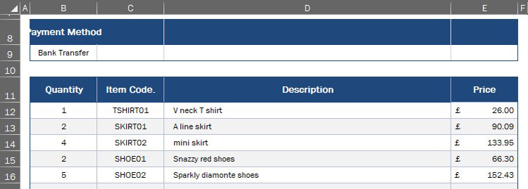
Finally, adding more product codes to our invoice gives us this clean result...

Now without product codes to our invoice gives us this tidy result...

You can download the excel files used to make this demo and try for yourself:

Price List Excel File: pricelist.xlsx

Invoice Excel File: invoice01.xlsx

Single Combined Excel File: combined.xlsx

We really hope this helps you to master Excel, but please let us know if you have any queries or comments about the above mini tutorial.